How to create a Heatmap

Downloading Data

For this session we are going to utilize the dataset from the https://encode.project.org/.

You can download the txt file here:

Install Packages and Loading Libraries

First step is to install packages either from CRAN, Bioconductor or from Github and to load the libraries.

library(data.table)
library(dplyr)
library(tidyverse)
library(plyr)
library(scales)
library(tidyquant)

Importing Data

Navigate your directory to your folder where you have saved the data set. Now we will go ahead to import our data set using the fread function.

my_data <- fread(filename)

Data wrangling

In order to have a clean data set we need to add column names and to remove the columns that are not needed for our final heatmap output.

colnames(my_data)[1:4] <- c("chrom","start","stop","type")
my_data <- my_data[,c(1:4)] #Keeping only the columns 1 to 4
my_data$type <- gsub('[[:digit:]]+_','',my_data$type) #removing the numbers and underscores from our type column
glimpse(my_data)

## Rows: 571,339
## Columns: 4
## $ chrom <chr> "chr1", "chr1", "chr1", "chr1", "chr1", "chr1", "chr1", "chr1", …
## $ start <int> 10000, 10600, 11137, 11737, 11937, 12137, 14537, 20337, 22137, 2…
## $ stop  <int> 10600, 11137, 11737, 11937, 12137, 14537, 20337, 22137, 22937, 2…
## $ type  <chr> "Repetitive/CNV", "Heterochrom/lo", "Insulator", "Weak_Txn", "We…

Split the data frame

We can now split our data frame by chromosome and type and apply a function summarizing the length for each type per chromosome using the ddply function from the plyr library.

my_data2 <- ddply(my_data, .(type, chrom), summarise , no = length(type))
glimpse(my_data2)

## Rows: 276
## Columns: 3
## $ type  <chr> "Active_Promoter", "Active_Promoter", "Active_Promoter", "Active…
## $ chrom <chr> "chr1", "chr10", "chr11", "chr12", "chr13", "chr14", "chr15", "c…
## $ no    <int> 1497, 596, 759, 788, 323, 498, 492, 668, 901, 243, 1085, 1011, 3…

Pivot_longer & Pivot_wider

pivot_longer() makes dataset longer by increasing the number of rows and decreasing the number of columns, whereas pivot_wider() is often utilized to tidy long data sets and often required for the purpose of the analysis (for example creating a heatmap)

my_data_final <- my_data2 %>% group_by(type) %>% 
  mutate(prop = no/sum(no)) %>% 
  ungroup() %>% 
  pivot_wider(
    id_cols = type,
    names_from = chrom,
    values_from = prop
  ) %>% arrange(-`chr19`) %>% 
  mutate(type = fct_reorder(type, `chr19`)) %>% 
  pivot_longer(
    cols = -type,
    names_to = "chrom",
    values_to = "prop"
  )

head(my_data_final)

## # A tibble: 6 × 3
##   type          chrom    prop
##   <fct>         <chr>   <dbl>
## 1 Weak_Enhancer chr1  0.0299 
## 2 Weak_Enhancer chr10 0.0151 
## 3 Weak_Enhancer chr11 0.0148 
## 4 Weak_Enhancer chr12 0.0158 
## 5 Weak_Enhancer chr13 0.00824
## 6 Weak_Enhancer chr14 0.0106

Creating a Heatmap

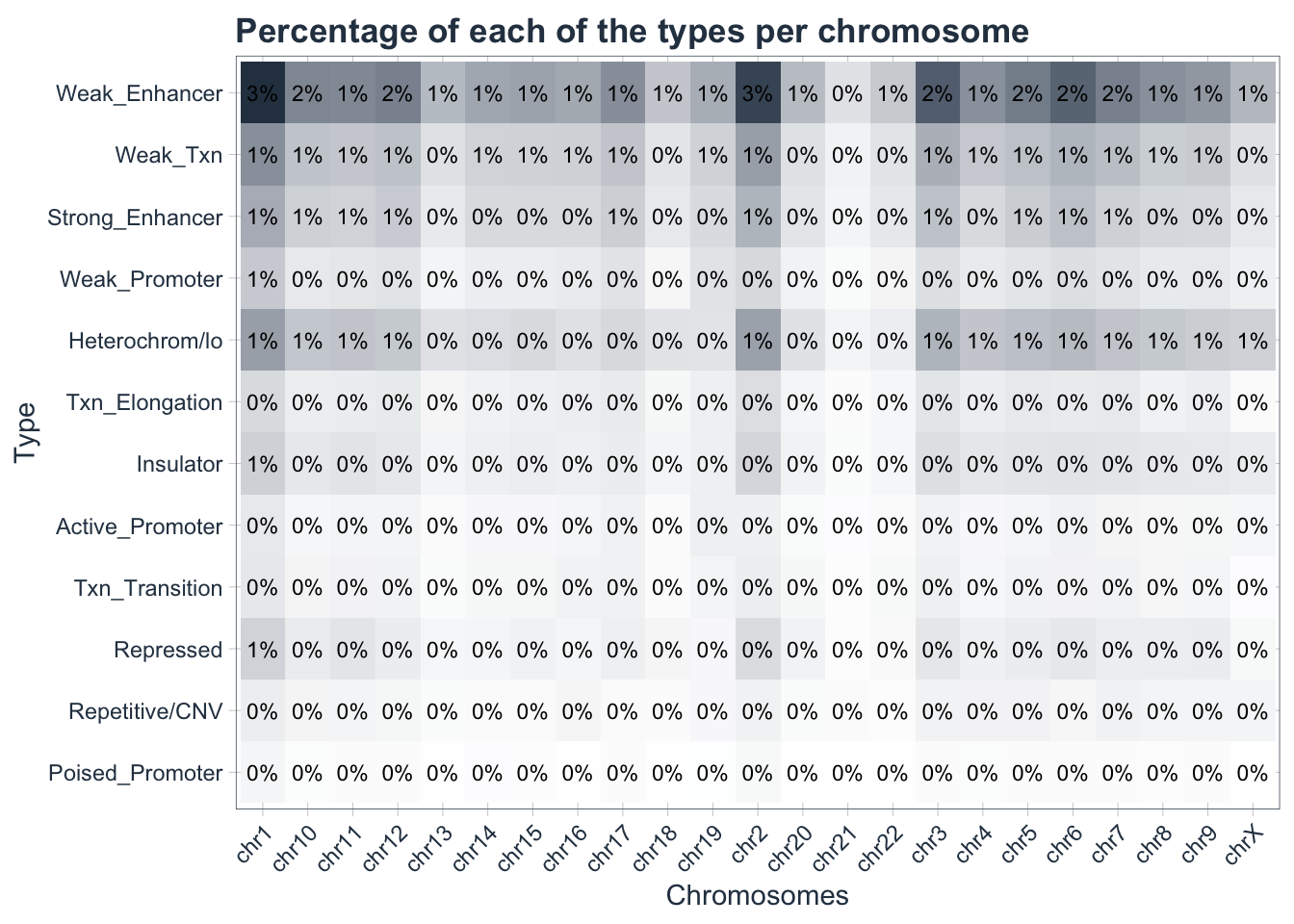
Finally we are ready to generate our first heatmap! One way to do that is to use the ggplot library.

heatmap <- my_data_final %>% 
ggplot(aes(chrom, type)) +
  geom_tile(aes(fill = prop)) +
  geom_text(aes(label = scales::percent(prop, accuracy = 1)),
            size = 3) +
  scale_fill_gradient(low = "white",high = palette_light()[1]) +
  labs(
    title = "Percentage of each of the types per chromosome",
    x = "Chromosomes",
    y = "Type"
  )+
  theme_tq() +
  theme(
    axis.text.x = element_text(angle = 45, hjust = 1),
    legend.position = "none",
    plot.title = element_text(face = "bold"))
    
  

    
heatmap